Application of Derivatives:Class 12 Maths NCERT Chapter 6

Key Features of NCERT Material for Class 12 Maths Chapter 6 – Application of Derivatives

In the previous Chapter 5:Continuity and Differentiability,we have learned about continuity, algebra of continuous function.In this Chapter 6:Application of derivatives we will learn about definition of derivatives, rate of change of quantities and many more.

Quick revision notes

Rate of Change of Quantities: Let y = f(x) be a function of x. Then, dy/dx speaks to the rate of change of y with respect to x. Additionally, (dy/dx)|x = x0 speaks to the rate of change of y with respect to x at x = x0. 

In the event that two variables x and y are differing with respect to another variable t, for example x = f(t) and y = g(t), at that point

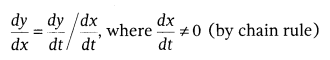
As it were, the rate of change of y with respect to x can be determined utilizing the rate of change of y and that of x both with respect to t. 

Note:  dy/dx is positive, if y increments as x increments and it is negative, if y diminishes as x increments, dx 

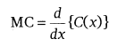
Marginal Cost: Marginal cost speaks to the prompt rate of change of the all out cost at any degree of yield. 

On the off chance that C(x) speaks to the cost function for x units created, at that point marginal cost (MC) is given by

Marginal Revenue: Marginal revenue speaks to the rate of change of all out revenue with respect to the quantity of things sold at a moment. 

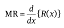
On the off chance that R(x) is the revenue function for x units sold, at that point marginal revenue (MR) is given by 

Leave I alone an open interval contained in the area of a genuine esteemed function f. At that point, f is supposed to be

• increasing on I, if x1 < x2 in I ⇒ f(x1) ≤ f(x2), ∀ x1, x2 ∈ I.
• strictly increasing on interval I, if x1 < x2 in I ⇒ f(x1) < f(x2), ∀ x1, x2 ∈ I.
• decreasing on I, if x1 < x2 in I ⇒ f(x1) ≥ f(x2), ∀ x1, x2 ∈ I.
• strictly decreasing on I, if x1 < x2 in f(x1) > f(x2), ∀ x1, x2 ∈ I.

Let x0 be a point in the space of meaning of a genuine esteemed function f, at that point f is supposed to be increasing, strictly increasing, decreasing or strictly decreasing at x0, if there exists an open interval I containing x0 with the end goal that f is increasing, strictly increasing, decreasing or strictly decreasing, respectively in I. 

Note: If for a given interval I ⊆ R, function f increment for certain qualities in I and reduction for different qualities in I, at that point we state function is neither increasing nor decreasing.

Let f be continuous on [a, b] and differentiable on the open interval (a, b). Then,

• f is increasing in [a, b] if f'(x) > 0 for each x ∈ (a, b).
• f is decreasing in [a, b] if f'(x) < 0 for each x ∈ (a, b).
• f is a constant function in [a, b], if f'(x) = 0 for each x ∈ (a, b).

Note:

(i) f is strictly increasing in (a, b), if f'(x) > 0 for each x ∈ (a, b).

(ii) f is strictly decreasing in (a, b), if f'(x) < 0 for each x ∈ (a, b).

Monotonic Function: A function which is either increasing or decreasing in a given interval I, is known as monotonic function.

Approximation: Let y = f(x) be any function of x. Let Δx be the little change in x and Δy be the relating change in y.

i.e. Δy = f(x + Δx) – f(x).Then, dy = f'(x) dx or dy = dy/dx Δx is a nice approximation of Δy, where dx = Δx is relatively small and we represent it by dy ~ Δy.

Note:

(I) The differential of the dependent variable isn’t equivalent to the augmentation of the variable while the differential of the independent variable is equivalent to the addition of the variable. 

(ii) Absolute Error : The change Δx in x is known as absolute error in x. 

Tangents and Normals

Slope: (i) The slope of a tangent to the curve y = f(x) at the point (x1, y1) is given by

(ii) The slope of a normal to the curve y = f(x) at the point (x1, y1) is given by

Note: If a tangent line to the curve y = f(x) makes an edge θ with X-axis in the positive direction, at that point =dy/dx Slope of the tangent = tan θ. dx

Equations of Tangent and Normal

The equation of tangent to the curve y = f(x) at the point P(x1, y1) is given by

y – y1 = m (x – x1), where we have m = dy/dx at point (x1, y1).

The equation of normal to the curve y = f(x) at the point Q(x1, y1) is given by

y – y1 =-1/m  (x – x1), where we have m =dy/dx  at point (x1, y1).

On the off chance that slope of the tangent line is zero, then tanθ = θ, so θ = 0, which implies that tangent line is parallel to the X-axis and then the equation of tangent at the point (x1, y1) is y = y1.

On the off chance θ → , then tanθ → ∞ which implies that tangent line is perpendicular to the X-axis, i.e. parallel to the Y-axis and at that point equation of the tangent at the point (x1, y1) is x = x0.

Maximum and Minimum Value:Let f be a function characterized on an interval I. At that point, 

(I) f is said to have a maximum incentive in I, if there exists a point c in I with the end goal that 

f(c) > f(x), ∀ x ∈ I. The number f(c) is known as the maximum estimation of f in I and the point c is known as a point of a maximum estimation of f in I. 

(ii) f is said to have a minimum incentive in I, if there exists a point c in I with the end goal that f(c) < f(x), ∀ x ∈ I. The number f(c) is known as the minimum estimation of f in I and the point c is known as a point of minimum estimation of f in I. 

(iii) f is said to have an extreme incentive in I, if there exists a point c in I with the end goal that f(c) is either a maximum worth or a minimum estimation of f in I. The number f(c) is canceled an extreme incentive in I and the point c is called an extreme point. 

Local Maxima and Local Minima 

(I) A function f(x) is said to have a local maximum incentive at point x = an, if there exists an area (a – δ, a + δ) of a with the end goal that f(x) < f(a), ∀ x ∈ (a – δ, a + δ), x ≠ a. Here, f(a) is known as the local maximum estimation of f(x) at the point x = a. (ii) A function f(x) is said to have a local minimum incentive at point x = an, if there exists an area (a – δ, a + δ) of a with the end goal that f(x) > f(a), ∀ x ∈ (a – δ, a + δ), x ≠ a. Here, f(a) is known as the local minimum estimation of f(x) at x = a. 

The points at which a function changes its inclination from decreasing to increasing or the other way around are called turning points.

Note: 

(I) Through the diagrams, we can even locate the maximum/minimum estimation of a function at a point at which it isn’t even differentiable. 

(ii) Every monotonic function assumes its maximum/minimum incentive at the endpoints of the domain of meaning of the function. 

Each continuous function on a shut interval has a maximum and a minimum worth.

Leave f alone a function characterized on an open interval I. Assume cel is any point. In the event that f has local maxima or local minima at x = c, at that point either f'(c) = 0 or f isn’t differentiable at c. 

Critical Point: A point c in the domain of a function f at which either f'(c) = 0 or f isn’t differentiable, is known as a critical point of f.

First Derivative Test: Let f be a function characterized on an open interval I and f be continuous of a critical point c in I. At that point ,

• on the off chance f'(x) changes sign from positive to negative as x increases through c, then c is a point of local maxima.
• on the off chance f'(x) changes sign from negative to positive as x increases through c, then c is a point of local minima.
• on the off chance f'(x) does not change sign as x increases through c, then c is neither a point of local maxima nor a point of local minima. Such a point is called a point of inflection.

Second Derivative Test: Let f(x) be a function characterized on an interval I and c ∈ I. Let f be twice differentiable at c. At that point,

(i) x = c is said to be a point of local maxima, if f'(c) = 0 and f”(c) < 0. (ii) x = c is said to be a point of local minima, if f'(c) = 0 and f”(c) > 0.

(iii) the test fails, if f'(c) = 0 and f”(c) = 0.

Note 

(I) If the test falls flat, at that point we return to the main derivative test and discover whether a will be a point of local maxima, local minima or a point of emphasis. 

(ii) If we state that f is twice differentiable at o, at that point it implies second request derivative exists at a. 

Absolute Maximum Value: Let f(x) be a function characterized in its domain say Z ⊂ R. Then, f(x) is said to have the maximum value at a point a ∈ Z, if f(x) ≤ f(a), ∀ x ∈ Z.

Absolute Minimum Value: Let f(x) be a function characterized in its domain say Z ⊂ R. Then, f(x) is said to have the minimum value at a point a ∈ Z, if f(x) ≥ f(a), ∀ x ∈ Z.

Note: Every continuous function characterized in a shut interval has a maximum or a minimum worth which lies either toward the end points or at the arrangement of f'(x) = 0 or at the point, where the function isn’t differentiable. 

Leave f alone a continuous function on an interval I = [a, b]. At that point, f has the absolute maximum worth and/accomplishes it in any event once in I. Likewise, f has the absolute minimum worth and accomplishes it at any rate once in I.